Google Sheets, part of the Google Workspace suite, is a powerful and user-friendly spreadsheet application that allows users to create, edit, and collaborate on spreadsheets online. One common task users encounter is checking whether a cell is empty or contains data. In this article, we will explore various methods to accomplish this task using functions, formulas, and conditional formatting. By the end, you’ll be well-equipped to efficiently manage and manipulate data in your Google Sheets.
Using ISBLANK Function
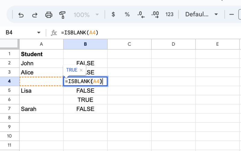
The ISBLANK function in Google Sheets checks if a specified cell is empty and returns either TRUE or FALSE based on the result. The syntax is as follows:
=ISBLANK(cell_reference)
Example: Suppose we have data in cell A1, and we want to check if it is empty. Use the following formula in any other cell:
=ISBLANK(A1)
If cell A1 is empty, the formula will return TRUE. Otherwise, it will return FALSE.
Using IF Function for Custom Output
You can combine the ISBLANK function with the IF function to display custom outputs based on whether a cell is empty or not. The syntax for the IF function is as follows:
=IF(logical_expression, value_if_true, value_if_false)
Example: Let’s use the IF function to display “Empty” when cell A1 is empty and “Not Empty” otherwise:
=IF(ISBLANK(A1), "Empty", "Not Empty")

Using COUNTA Function
The COUNTA function counts the number of non-empty cells within a given range. By using this function, you can indirectly check if a cell is empty or not. The syntax is as follows:
=COUNTA(cell_range)
Example: Suppose we want to check if cells A1 to A5 are empty. Use the COUNTA function like this:
=IF(COUNTA(A1:A5) = 0, "All Empty", "Some Non-empty")
This formula will return “All Empty” if all cells in the range are empty; otherwise, it will return “Some Non-empty.”
Using Conditional Formatting
Conditional formatting in Google Sheets allows you to apply different formatting styles based on specific conditions. You can use this feature to visually identify empty cells easily.
Example: To apply conditional formatting to cell A1, follow these steps:
- Select cell A1.
- Go to Format > Conditional formatting.
- In the conditional format rules panel, choose “Custom formula is” from the dropdown menu.
- Enter the formula
=ISBLANK(A1)in the input field. - Choose the desired formatting style for empty cells.
- Click “Done.”
Now, whenever cell A1 is empty, it will be formatted according to your chosen style, making it stand out visually.
Conclusion
In this article, we explored different methods to check if a cell is empty in Google Sheets. Whether you prefer using functions like ISBLANK, IF, or COUNTA, or you opt for the visual approach with conditional formatting, you can easily manage and analyze your data. By mastering these techniques, you can efficiently handle empty cells and make more informed decisions in your spreadsheets. Happy data managing!
