
INDEX MATCH in Google Sheets is a combination of two functions: INDEX and MATCH. INDEX returns a value from the intersection of a specified row and a specified column within an array, while MATCH searches for an item in an array and returns its position. When used together, INDEX MATCH has several advantages over VLOOKUP, improving on its limitations to help you find data more quickly and accurately. INDEX MATCH can search through horizontal and vertical ranges, return approximate results when searching for text, and look up data on the left side of the target cell. Furthermore, INDEX MATCH can even lookup values from multiple sheets or workbooks with the same function name and syntax. INDEX MATCH is easy to learn and apply and requires only a few keystrokes – so take advantage of it today instead of relying solely on VLOOKUP when you need to locate a certain record!
Google Sheets INDEX function
INDEX MATCH is 2 functions that when used together produce the desired result. To understand how to use this feature, you need to understand the syntax of both functions. Speaking of the INDEX function, it is needed to extract the very value of the searched row in the entire table.
=INDEX(reference,
, [column])
- Reference is the range to be searched. It is mandatory.
- Row – allows you to specify the number of offset rows to be processed. The countdown starts from the first cell in the range. You can not specify, the default value is 0.
- Column is another optional formula parameter that can be ignored. Same as Row but refers to the number of offset columns.
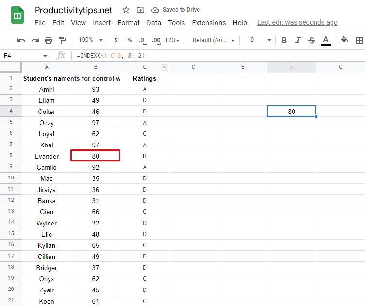
Here is the simplest example. As a result of executing the formula, the function will return the value of cell 8 in the second column of the specified range.
=INDEX(A1:C10, 8, 2)
Google Sheets MATCH function
The MATCH function performs the opposite action, namely, it looks up the specified value in the table.
=MATCH(search_key, range, [search_type])
- Search_key is the same value to be found in the entry. It is a required parameter.
- Range – passes the range in which to search for the formula. The same applies to mandatory parameters.
- Search_type – indicates the type of search: exact or approximate. If you specify 1, the function will sort your range in ascending order. Provided that the desired value is not in the sample, the output will give the most approximate number. A value of 0 will tell the function to look up the exact value. You can also pass -1, then sorting will be in descending order.
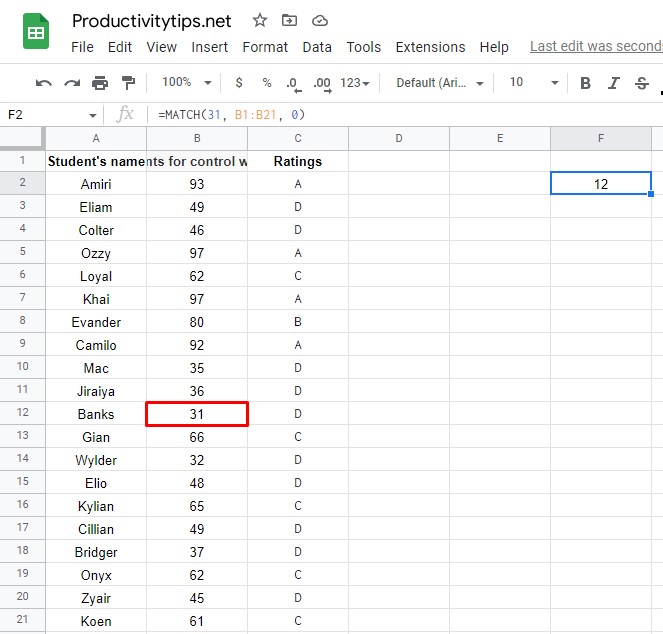
For example, using MATCH we want the sequence number of the student who scored the lowest score.
=MATCH(31, B1:B21, 0)
How to Use INDEX MATCH in Google Sheets?
To understand how it all works together, we’ll take a simple example. Our goal is to find the student who failed the test. Knowing his score (or score), you need to find the name of the failed one.
- We are looking for the line number of a student who received an E grade.
=MATCH(“E”, C1:C21,0)
- We expand the search range and pass the location of the problem student to the formula.
=INDEX(A1:C21, MATCH(“E”, C1:C21,0))
- We indicate which parameter related to this student we are interested in. In this case, the name is in the first column.
=INDEX(A1:C21, MATCH(“E”, C1:C21,0), 1)

There are many uses for INDEX MATCH in Google Sheets. This is a more advanced search option compared to VLOOKUP, since you can take into account the case of the text, there is an operator with the ability to search for approximate values, left-hand search is available. You’ll have to experiment a little and all the possibilities of INDEX MATCH will open before you in all their glory.