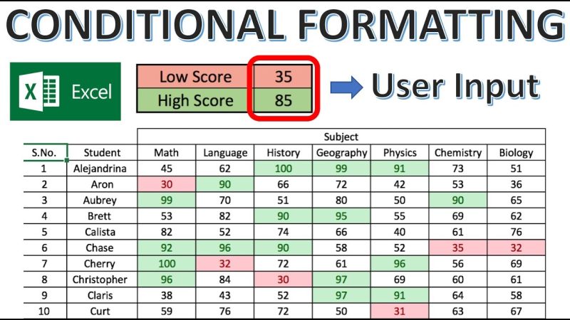
Conditional formatting in Google Sheets is a powerful tool that can easily help you sort through a lot of data. You can have the cell format based on conditions you select—for example, if one cell contains a value higher than 10, you can make it bold or change its color to highlight it as important. You can also apply the same formatting to an entire range of cells if they meet specific criteria. The possibilities don’t stop there; you can even set the formatting based on conditions met in another cell! By leveraging this feature for your own spreadsheets, you will be able to better analyze and interpret your data quickly and easily.
How to Use Google Sheets Conditional Formatting?
Learning how to use conditional formatting can help you draw attention to key data points quickly. All that’s required is to choose what format should be applied based on a value or expression, whether it’s a cell reference or other numerical value. Do this for each data set, and in an instant you’ll have an easy way to view the performance of your website at a glance!
How to use Google Sheets conditional formatting:
- Select the cell to be formatted.
- Click on the “Format” tab on the navigation bar and select “Conditional Formatting”.
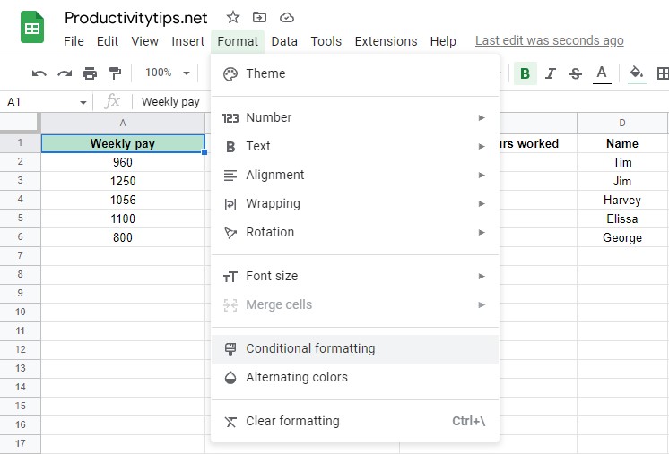
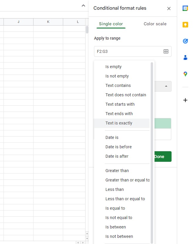
- Set the formatting rules you want.
- If you need to use a formula for conditional formatting, then go to the “Format cells if…” section and set the correct formatting rules.
- After selecting the style, click on the “Finish” button.
Advice! You can check your rules in the “Conditional Formatting Rules” section. Here you will also see all the formatting rules that are currently active in your table.
How to Use Google Sheets Conditional Formatting Based on Another Column?
By understanding the basics of the function, you will be able to perform Conditional formatting based on another cell value.
How to use Google Sheets conditional formatting based on another column:
- Select the cell to be formatted.
- On the “Format” tab, look for the “Conditional Formatting” section and click on it.
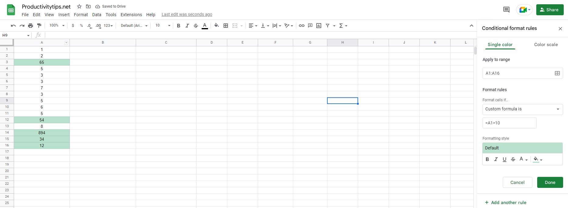
- In the Formatting Rules section, click on Custom Formula.
- Enter your formula and click on the “Finish” button.
Conclusion
How conditional formatting works is quite simple if you know how to use at least the basic functions of Google Sheets. As a condition, you can use both standard and custom functions. For comparison, you can use values, text, dates. A color or other cell style cannot be used as an input. This information is enough to make full use of conditional formatting.