Have you ever needed to extract the domain from a URL in your Google Sheets? Whether you’re working on a data analysis project or simply organizing website links, knowing how to extract the domain from URLs can save you valuable time and effort. In this article, we’ll guide you through a step-by-step process on how to accomplish this task effectively using Google Sheets functions.
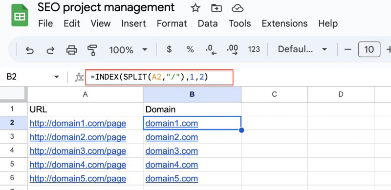
=INDEX(SPLIT(A2,“/”),1,2)
Step 1: Understanding the URL Structure
Before we dive into the extraction process, let’s briefly understand the typical structure of a URL. A URL (Uniform Resource Locator) is composed of several parts, such as the protocol (e.g., “https://” or “http://”), the domain name (e.g., “example.com”), the path (optional), and query parameters (optional). For this article, we’ll focus on extracting the domain name.
Step 2: Using the “Split” Function
The “Split” function in Google Sheets allows us to divide a string into separate parts based on a specified delimiter. Since URLs are usually delimited by slashes (“/”), we can use this function to extract the domain.
Let’s say cell A1 contains the URL you want to extract the domain from. To do this, follow these steps:
- In cell B1, enter the following formula:
=SPLIT(A1, "/")
- Press “Enter.” Now, cell B1 will show the domain name and other URL components in separate columns.
Step 3: Retrieving the Domain Name
Now that we have the URL components separated, we can isolate the domain name. The domain name will typically be in the third column (index 2) after splitting the URL.
To extract the domain name, enter the following formula in cell C1:
=INDEX(B1, 1, 3)
After pressing “Enter,” cell C1 will display the domain name without any other URL components.
Step 4: Handling Subdomains
The above method works well for URLs with simple domain names like “example.com.” However, some URLs might have subdomains like “subdomain.example.com.” In such cases, the domain name may appear in the fourth column (index 3) after splitting the URL.
To account for subdomains, you can modify the formula in cell C1 as follows:
=IFERROR(INDEX(B1, 1, 3), INDEX(B1, 1, 4))
The modified formula checks if the third column contains data (domain name without subdomain). If it doesn’t, the formula will return the domain name from the fourth column, considering it as a subdomain scenario.
Step 5: Cleaning Up the Domain Name
Sometimes, the domain name might include additional elements like “www” or “https://”. To clean up the domain, you can use the “SUBSTITUTE” function to remove these prefixes.
In cell D1, enter the following formula:
=SUBSTITUTE(C1, "www.", "")
This formula will remove any occurrence of “www.” from the domain name, leaving you with a clean representation.
Conclusion
Extracting domain names from URLs in Google Sheets can be achieved through a series of simple functions. By utilizing the “SPLIT” function and adjusting for subdomains, you can efficiently manage and organize your data. Remember to apply the “SUBSTITUTE” function if you want to further clean up the domain names. Now you can confidently work with URLs in Google Sheets without any hassle. Happy spreadsheeting!