If you’re like most people, you probably use Google Sheets to keep track of data. Whether it’s a grocery list or a list of tasks to complete, Sheets is a great way to organize information. But sometimes, the gridlines that appear by default can be a bit distracting. This is a small problem, because they are easy to get rid of. Here is the instruction how to hide gridlines in Google Sheets.
How to Hide Gridlines in Google Sheet?
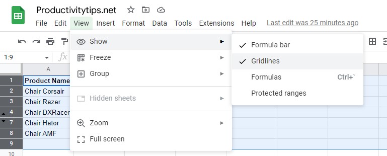
To remove gridlines in Google Sheets, follow these steps:
- Open your Google Sheet.
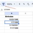
- Select the View menu.
- Click on gridlines.
Your gridlines should now be hidden! If you want to show them again, simply follow the same steps. You can also adjust the thickness and color of your gridlines by going to Format > Cells > Border > More options. From here, you can select the thickness, color, and style of your border. Experiment with different combinations until you find one that you like!
How to Get Rid of Gridlines in Google Sheet when printing?
If you’re only concerned about gridlines in Google Sheets when you print your document, you can turn them off just before you print. That is, they will appear in the virtual document, but will be ignored when printed onto a sheet of paper.
For this you need:
- Select the cells that you will print.
- Click on the “File” tab and click on the “Print” button.
- Remove the flag from the “Show grid lines” checkbox.

That’s it! Now you know how to hide gridlines in Google Sheets, both in the virtual document and when printing. If you have any questions or comments, please feel free to leave them in the space below.