If you’ve ever tried to enter a formula into a cell in Google Sheets and gotten an error message, you’re not alone. The “formula parse error” is a common problem that can occur for a number of reasons. Fortunately, there are a few simple steps you can take to fix the problem.
What is a Formula Parse Error in Google Sheets?
Formula parse error google sheets is caused when the formula submitted is not able to be parsed correctly by the software. There are many different reasons this can happen, such as a typo in the formula, incorrect cell references, or trying to do an impossible calculation. All of these formula parse errors will generally result in the same error message being displayed. However, depending on the type of parse error formula encountered, there might be some slight variations in the message.
How to fix different types of Formula Parse Error?
Error messages are not always easy to understand, but we have provided some clarification below on a few of the most common messages that you might encounter. With this information, you should be able to identify and fix formula parse errors in your own spreadsheet with ease!
#N/A Error
The #N/A error is a common error when using lookup formulas in Google Sheets. The error simply means that the value you are looking for is not available. This problem often occurs when you are looking for a value that does not exist in the given range. For example, if you use the VLOOKUP function to find a value from a range and that value does not exist, you will see a #N/A error.
To fix this problem, you can either check the range for the missing value or use a different function. If you are using VLOOKUP, you can try using the IFERROR function to handle the #N/A error. The IFERROR function will return a value if there is no error and return an alternate value if there is an error. For example, you could use IFERROR to return a 0 if there is an error. This would allow the VLOOKUP function to continue working even if there are missing values.
#DIV/0 Error
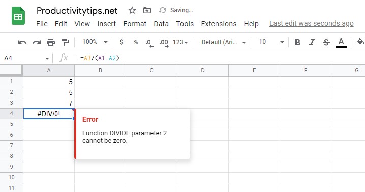
This error occurs when a number in the formula is being divided by zero. This makes no sense mathematically, so the function returns a #DIV/0 error. There are a few reasons why this error might occur. For example, if you are trying to divide a value by a function or operation that results in a 0 value, you will get a #DIV/0 error.
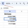
In the image below, we are trying to divide the number 7 by the difference between values in A1 and A2, which results in 0. Since it is not possible to divide 7 by 0, the formula returns a #DIV/0 error.
This error also happens when you are trying to apply the AVERAGE function on a range of blank cells. This happens as the AVERAGE function needs to divide the SUM of the values with the number of the values, and if the range is blank, it’s equivalent to dividing by 0.
The good news is that this error can be easily fixed. All you need to do is add a check for 0 values before performing the division. For example, you can use the IFERROR function to catch #DIV/0 errors and replace them with something else. Alternatively, you can also use conditional formatting to highlight cells that contain #DIV/0 errors. This will help you identify and fix these errors quickly and easily.
#REF! Error
The #REF! error in Google Sheets appears when your formula has an invalid reference. There are two main types of invalid references: missing references and circular dependencies. Missing references occur when you try to reference a cell that no longer exists, while circular dependencies occur when your formula references itself. To fix a #REF! error, you need to identify the invalid reference and correct it. In the case of a missing reference, this may mean adding back the missing cell or changing the cell reference in your formula. For a circular dependency, you need to adjust your formula so that it no longer references itself. Once you have corrected the invalid reference, your #REF! error should disappear.
#VALUE! Error
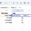
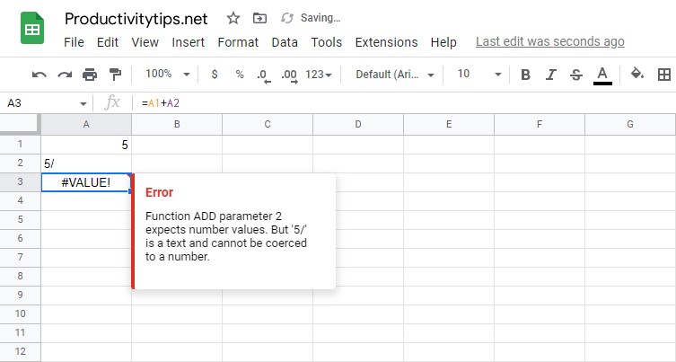
Google Sheets Error: #VALUE! occurs when one or more parameters in your formula are of a different type than what is expected. So if a function only accepts numbers as a parameter, but you have a text value in the cell being referenced, then you will end up with a #VALUE! error. In the image below, a backslash character (\) got added to the end of the number in cell A2 by mistake. So when we use the formula =A1+A2 in cell A3, we are trying to add a number to a text value, which is invalid. Therefore, the formula returns a #VALUE! Error.
#NAME? Error
The #NAME? error can occur for a number of reasons. One common cause is a problem with the syntax of your formula. This could be due to a spelling mistake, an incorrect named range, or the presence or absence of quotation marks. For example, if you forget to add quotation marks around a string value, then the formula considers it as a named range. If a named range by that name doesn’t exist, then it returns a #NAME? Error.
Another common reason for the #NAME? error is when Excel cannot recognize a function or command. This can happen if you are using a custom function or macro that is not installed on your computer. If you are using a custom function or macro, make sure that it is installed properly and that you have entered the correct syntax.
You may also see the #NAME? error if you are trying to use a feature that is not available in your version of Excel. For example, the FILTER function was introduced in Excel 2016, so if you are using an earlier version of Excel, you will get the #NAME? error if you try to use FILTER in your formulas. To fix this problem, either update to the latest version of Excel or use an alternative function that is available in your version of Excel.
Finally, the #NAME? error can also occur if there are spaces or non-printable characters in your cell references. Cell references must begin with an equal sign (=), and they cannot contain any spaces or non-printable characters such as tabs or carriage returns. If your cell reference does contain spaces or non-printable characters, you will need to remove them before the formula will work correctly.
#NUM! Error
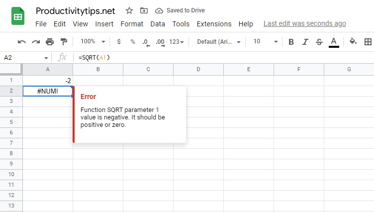
#NUM! errors in Google Sheets occur when your formula has invalid numeric values. This may happen if you try to take the square root of a negative number, or if a calculation results in a very large number that is outside the scope of what Google Sheets can handle. For example, we are passing a negative value to the SQRT function, which is not acceptable, so the function returns a #NUM! error.
#ERROR! Message
The #ERROR! Message is a specific error that appears in Google Sheets. This error occurs when the Google Sheets program is unable to interpret a formula. There can be many reasons for this error to occur, such as forgetting to add an important operator between cell references, values, or parameters. Another reason this error might occur is if the number of opening brackets does not match the number of closing brackets in a formula. For example, if a formula includes a $ symbol to refer to a price amount, but Google Sheets mistake it for an absolute reference, the formula will not make sense and the #ERROR! Message will appear. Troubleshooting this error can be difficult, but it is important to try various methods until the correct solution is found.
This article will show you how to fix formula parse errors in Google Sheets so that you can get back to work. The first step is to check your formulas for any syntax errors. Next, make sure that your cells are referencing the correct range of cells. Finally, check your cell references for any typos. If you follow these steps, you should be able to fix most formula parse errors in Google Sheets.