How to use VLOOKUP from Another Sheet in Google Sheets?

One of the most powerful features of Google Sheets is the Vlookup function. Vlookup stands for “vertical lookup,” and it allows you to quickly find specific values in large data sets. While Vlookup is incredibly useful on a single sheet, you can further enhance its power by using it to call data from other spreadsheets. This can be especially helpful if you have a large data set that spans multiple sheets. With Vlookup, you can lookup and fetch specific values from these other sheets quickly and easily. This can save you hours of work, and it also helps to keep your data clean and up-to-date. So if you’re looking for a quick and easy way to enhance your data analysis, consider using the Vlookup function in Google Sheets.

VLOOKUP Function Syntax

Vlookup is a function in Excel that allows you to search for a specific value in a range of cells and return the value from a different cell in the same row. The syntax for Vlookup is pretty straightforward, but it can be used to a highly complex degree.

=Vlookup(search_value, table_array, col_index_num, [range_lookup])

The function takes four arguments: 

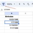
• search_value – this is the value that you want to look up, i.e. the value in cell A1. The lookup_value can be a number, text string or even a cell reference to a value.
• table_array – this is where you tell Vlookup which cells contain the data you want to search through and ultimately return a result from. Usually this will be another worksheet or even another workbook altogether. If this is the case then you need to use the workbook name and worksheet name before your named range like this:[workbook name]![worksheet name]!mynamedrange . You could also have used a named range here too instead of an exact cell reference like we have done i.e. mynamedrange instead of B1:C10.
• col_index – once Vlookup has found a match based on your lookup value it needs to know which column in your table array contains the data that you want returned, i.e. the ID number corresponding with the name that was input in cell A1 of Sheet 1. The way Vlookup does this is by means of an index number starting at 1 for the leftmost column through to whatever number corresponds with the column containing your required data further to the right of your table array (remembering that it can only search right). 
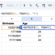
• [range _ lookup] – this last part of the formula is optional but there are two values that you can use here; either TRUE or FALSE . If you don’t specify anything then by default it will assume that you want an approximate match , i.e TRUE , so if it can’t find an exact match then it will return whatever value is closest below it in your range C1:C10 . If on the other hand you wanted an EXACT match only then specify FALSE for this parameter like this: =VLOOKUP(A1,B1:C10,2,,FALSE) otherwise leave it blank like above and let Excel work its magic!  

How to use VLOOKUP in the Same Workbook and in a Different Workbook?

The VLOOKUP function in Google Sheets is incredibly versatile and can be used to lookup data in a variety of different scenarios. While most of the time we use the function on the same sheet, there are times when you may need to use it to lookup data on a different sheet or even in a different workbook.

For example, you may want to fetch data from specific items in a worksheet but the lookup data is located in a different sheet or workbook. In this case, you would need to use the VLOOKUP formula to bring in the data from the other sheet or workbook.

The formula for using VLOOKUP between two sheets in the same workbook is slightly different than when you’re working with a different workbook. When working within the same workbook, you would use the following formula:

=VLOOKUP(lookup_value,sheet_name!range,col_index_num,FALSE)

For example, if you wanted to fetch data about specific items in Sheet1 and the lookup data was located in Sheet2, your formula would look like this:

=VLOOKUP(A2,Sheet2!A:B,2,FALSE)

On the other hand, if you wanted to fetch data from a different workbook altogether, your formula would look like this:

=VLOOKUP(lookup_value,'[workbook name]sheet name’!range,col_index_num,FALSE)

For example, if you wanted to fetch data from Sheet1 in Workbook1 and lookup data was located in Sheet2 of Workbook2, your formula would look like this: =VLOOKUP(A2,'[Workbook2]Sheet2′!A:B’,2),FALSE)

As you can see, using VLOOKUP to fetch data from another sheet or workbook is relatively straightforward. Just remember to adjust your formula accordingly depending on whether you’re working with sheets in the same workbook or not. By leveraging the power of VLOOKUP , you can easily get the data you need from wherever it’s located.

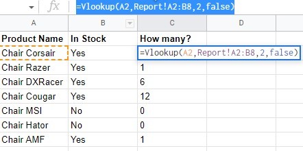
Vloop example

If you need to use data from another page of the same document, the following formula will work for you:

=Vlookup(A2,Report!A2:B8,2,false)

You only need to substitute your input and everything will work. The formula will be slightly different if the data needs to be obtained from another document. Here you will also need an importrange statement and a link. Be sure the second document must have the appropriate access. The formula looks like this:

=Vlookup(A2,importrange(“https://docs.google.com/spreadsheets/d/1P-mXCU2u9t621tq8oJmE8vFAvDabQznRqaMNTxxoSLw”,”Report!A2:B8″),2,false)

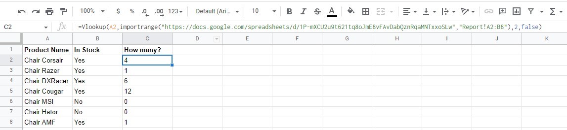
Of course, you need to put your link, tab name and range. If it doesn’t work the first time, check the syntax is correct. It is important to close the brackets in the right place.